- Blog
- AI & ML Expertise
- Introduction to Python for Statistical Learning
Introduction to Python for Statistical Learning
The first session in our statistical learning with Python series will briefly touch on some of the core components of Python’s scientific computing stack that we will use extensively later in the course. We will not only introduce two important libraries for data wrangling, numpy and pandas, but also show how to create plots using matplotlib. Please note that this is not a thorough introduction to these libraries; instead, we would like to point out what basic functionality they provide and how they differ from their counterparts in R.
But before we get into the details we will briefly describe how to setup a Python environment and what packages you need to install in order to run the code examples in this notebook.
Requirements
Python environment
We strongly recommend that you use a bundled Python distribution such as Anaconda. We have assembled a quick installation guide for Mac, Linux, and Windows in a previous blog post.
To run the R examples in this code you also need:
rpy2>=2.3.1You can find instructions how to install rpy2 here . If you have an working R environment on your machine the following command should install rpy2:
$ pip install -U rpy2To test if rpy2 was installed correctly run:
$ python -m 'rpy2.tests'If you run on Anaconda and it complains that it misses libreadline.so please install the following conda package:
$ conda install python=2.7.5=2IPython
IPython is an interactive computing environment for Python. It is a great tool for interactive data analysis and programming in general. Amongst other things it features a web-based notebook server that supports code, documentation, inline plots, and much more. In fact, all blog posts in this series will be written using IPython notebooks with the advantage that you can simply download it from here and either run it locally or view it on nbviewer.
Manipulating Data
The goal of this session is to get familiar with the basics of how to work with data in Python. The basic data containers that are used to manipulate data in Python are n-dimensional arrays that act either as vectors, matrices, or tensors.
In contrast to statistical computing environments like R, the fundamental data structures for data analysis in Python are not built into the computing environment but are available via dedicated 3rd party libraries. These libraries are called numpy and pandas.
Numpy
Numpy is the lingua-franca in the Python scientific computing ecosystem. It basically provides an n-dimensional array object that holds elements of a specific dtype (eg. numpy.float64 or numpy.int32). Most packages that we will discuss in this series will directly operate on arrays. Numpy also provides common operations on arrays such as element-wise arithmetic, indexing/slicing, and basic linear algebra (dot product, matrix decompositions, …).
Below we show some basic working with numpy arrays:
In [36]:
from __future__ import division  # always use floating point division
import numpy as np  # convention, use alias ``np``

# a one dimensional array
x = np.array([2, 7, 5])
print 'x:', x  # print x

# a sequence starting from 4 to 12 with a step size of 3
y = np.arange(4, 12, 3)
print 'y:', y

# element-wise operations on arrays
print 'x + y:', x + y
print 'x / y:', x / y
print 'x ^ y:', x ** y  # python uses ** for exponentiation
x: [2 7 5]
y: [ 4 7 10]
x + y: [ 6 14 15]
x / y: [ 0.5 1. 0.5]
x ^ y: [ 16 823543 9765625]If you need any help on operations such as np.arange you can access its documentation by either typing help(np.arange) or — if you use IPython — write a '?' after the command: np.arange?.
You can index and slice an array using square brackets []. To slice an array, numpy uses Python’s slicing syntax x[start:end:step] where step is the step size which is optional. If you omit start or end it will use the beginning or end, respectively. Python uses exclusive semantics meaning that the element with position end is not included in the result. Indexing can be done either by position or by using a boolean mask:In [37]:
print x[1]  # second element of x
print x[1:3]  # slice of x that includes second and third elements
print
print x[-2]  # indexing using negative indices - starts from -1
print x[-np.array([1, 2])]   # fancy indexing using index array
print

print x[np.array([False, True, True])]  # indexing using boolean mask
7
[7 5]
7
[5 7]
[7 5]For two or more dimensional arrays we just add slicing/indexing arguments, to select the whole dimension you can simply put a colon (:).In [38]:
# reshape sequence to 2d array (=matrix) where rows hold contiguous sequences
# then transpose so that columns hold contiguous sub sequences
z_temp = np.arange(1, 13).reshape((3,4))
print "z_temp"
print z_temp
print

# transpose
z = z_temp.T
print "z = z_temp.T (transpose of z_temp)"
print z
print

# slicing along two dimensions
a = z[2:4, 1:3]
print "a = z[2:4, 1:3]"
print a
print

# slicing along 2nd dimension
b = z[:, 1:3]
print "b = z[:, 1:3]"
print b
print

# first column, returns 1d array
c = z[:, 0]
print "c = z[:, 0]"
print c # one dimensional
print

# first column but return 2d array (remember: exclusive semantics)
cc = z[:, 0:1]
print "cc = z[:, 0:1]"
print cc  # two dimensional; column vector
z_temp
[[ 1 2 3 4]
[ 5 6 7 8]
[ 9 10 11 12]]
z = z_temp.T (transpose of z_temp)
[[ 1 5 9]
[ 2 6 10]
[ 3 7 11]
[ 4 8 12]]
a = z[2:4, 1:3]
[[ 7 11]
[ 8 12]]
b = z[:, 1:3]
[[ 5 9]
[ 6 10]
[ 7 11]
[ 8 12]]
c = z[:, 0]
[1 2 3 4]
cc = z[:, 0:1]
[[1]
[2]
[3]
[4]]To get information on the dimensionality and shape of an array you will find the following methods useful:
In [39]:
print z.shape  # number of elements along each axis (=dimension)
print z.ndim  # number of dimensions

print z[:, 0].ndim  # return first column as 1d array
(4, 3)
2
1In numpy, slicing will return a new array that is basically a view on the original array, thus, it doesn’t require copying any memory. Indexing (in numpy often called fancy indexing), on the other hand, always copies the underlying memory.

Differences between R and Python
R differentiates between vectors and matrices whereas in numpy both are unified by the n-dimensional numpy.ndarray class. There are a number of crucial differences in how indexing and slicing are handled in Python vs. R.
Note that the examples below require the Python package rpy2 to be installed.In [66]:
# allows execution of R code in IPython
try:
    %load_ext rmagic
except ImportError:
    print "Please install rpy2 to run the R/Python comparision code examples"
The rmagic extension is already loaded. To reload it, use:
%reload_ext rmagicPython uses 0-based indexing whereas indices in R start from 1:In [41]:
x = np.arange(5)  # seq has excl semantics
x[0]
Out[41]:
0In [65]:
%%R  # tells IPython that the following lines will be R code
x <- seq(0, 4)  # seq has incl semantics
print(x[1])
[1] 0Python uses exclusive semantics for slicing whereas R uses inclusive semantics:In [43]:
x[0:2] # doesnt include index 2Out[43]:
array([0, 1])In [44]:
%%R
x <- seq(0, 4)  # seq has incl semantics
print(x[1:2])  # includes index 2
[1] 0 1Negative indices have different semantics: in Python they are used to index from the end on an array whereas in R they are used to drop positions:In [45]:
x[-2] # second element from the endOut[45]:
3In [46]:
%%R
x <- seq(0, 4)  # seq has incl semantics
print(x[-2])  # drop 2nd position, ie 1
[1] 0 2 3 4If you index on a specific position of a matrix both R and Python will return a vector (ie. array with one less dimension). If you want to retain the dimensionality, R supports a drop=FALSE argument whereas in Python you have to use slicing instead:
In [47]:
X = np.arange(4).reshape((2, 2)).T  # 2d array
X[0:1, :]  # still 2d array - slice selects one element
Out[47]:
array([[0, 2]])In [48]:
%%R
X = matrix(seq(0, 3), 2, 2)
print(X[1, , drop=FALSE])  # use drop=FALSE
[,1] [,2]
[1,] 0 2Pandas
As numpy, pandas provides a key data structure: the pandas.DataFrame; as can be inferred from the name it behaves very much like an R data frame. Pandas data frames address three deficiencies of arrays:
- they hold heterogenous data; each column can have its own
numpy.dtype, - the axes of a DataFrame are labeled with column names and row indices,
- and, they account for missing values which this is not directly supported by arrays.
Data frames are extremely useful for data munging. They provide a large range of operations such as filter, join, and group-by aggregation.
Below we briefly show some of the core functionality of pandas data frames using some sample data from the website of the book “Introduction to Statistical Learning”:
In [49]:
import pandas as pd  # convention, alias ``pd``

# Load car dataset
auto = pd.read_csv("https://www-bcf.usc.edu/~gareth/ISL/Auto.csv")
auto.head()  # print the first lines
Out[49]:
| № | mpg | cylinders | displacement | horsepower | weight | acceleration | year | origin | name |
|---|---|---|---|---|---|---|---|---|---|
| 0 | 18 | 8 | 307 | 130 | 3504 | 12.0 | 70 | 1 | chevrolet chevelle malibu |
| 1 | 15 | 8 | 350 | 165 | 3693 | 11.5 | 70 | 1 | buick skylark 320 |
| 2 | 18 | 8 | 318 | 150 | 3436 | 11.0 | 70 | 1 | plymouth satellite |
| 3 | 16 | 8 | 304 | 150 | 3433 | 12.0 | 70 | 1 | amc rebel sst |
| 4 | 17 | 8 | 302 | 140 | 3449 | 10.5 | 70 | 1 | ford torino |
One of the first things you should do when you work with a new dataset is to look at some summary statistics such as mean, min, max, the number of missing values and quantiles. For this, pandas provides the convenience method pd.DataFrame.describe:
In [50]:
auto.describe()Out[50]:
| . | mpg | cylinders | displacement | weight | acceleration | year | origin |
|---|---|---|---|---|---|---|---|
| count | 397.000000 | 397.000000 | 397.000000 | 397.000000 | 397.000000 | 397.000000 | 397.000000 |
| mean | 23.515869 | 5.458438 | 193.532746 | 2970.261965 | 15.555668 | 75.994962 | 1.574307 |
| std | 7.825804 | 1.701577 | 104.379583 | 847.904119 | 2.749995 | 3.690005 | 0.802549 |
| min | 9.000000 | 3.000000 | 68.000000 | 1613.000000 | 8.000000 | 70.000000 | 1.000000 |
| 25% | 17.500000 | 4.000000 | 104.000000 | 2223.000000 | 13.800000 | 73.000000 | 1.000000 |
| 50% | 23.000000 | 4.000000 | 146.000000 | 2800.000000 | 15.500000 | 76.000000 | 1.000000 |
| 75% | 29.000000 | 8.000000 | 262.000000 | 3609.000000 | 17.100000 | 79.000000 | 2.000000 |
| max | 46.600000 | 8.000000 | 455.000000 | 5140.000000 | 24.800000 | 82.000000 | 3.000000 |
You can use the dot . or bracket [] notation to access columns of the dataset. To add new columns you have to use the bracket [] notation:
In [51]:
mpg = auto.mpg  # get mpg column
weight = auto['weight']  # get weight column
auto['mpg_per_weight'] = mpg / weight

print auto[['mpg', 'weight', 'mpg_per_weight']].head()
mpg weight mpg_per_weight
0 18 3504 0.005137
1 15 3693 0.004062
2 18 3436 0.005239
3 16 3433 0.004661
4 17 3449 0.004929Columns and rows of a data frame are labeled, to access/manipulate the labels either use pd.DataFrame.columns or pd.DataFrame.index:
In [52]:
print(auto.columns)
print(auto.index[:10])
Index([u'mpg', u'cylinders', u'displacement', u'horsepower', u'weight', u'acceleration', u'year', u'origin', u'name', u'mpg_per_weight'], dtype=object)
Int64Index([0, 1, 2, 3, 4, 5, 6, 7, 8, 9], dtype=int64)Indexing and slicing work similar as for numpy arrays just that you can also use column and row labels instead of positions:
In [53]:
auto.ix[0:5, ['weight', 'mpg']] # select the first 5 rows and two columns weight and mpgOut[53]:
| № | weight | mpg |
|---|---|---|
| 0 | 3504 | 18 |
| 1 | 3693 | 15 |
| 2 | 3436 | 18 |
| 3 | 3433 | 16 |
| 4 | 3449 | 17 |
| 5 | 4341 | 15 |
For more information on pandas please consult the excellent online documentation or the references at the end of this post.
Differences between R and Python
The major difference between the data frame in R and pandas from a user’s point of view is that pandas uses an object-oriented interface (ie methods) whereas R uses a functional interface:
In [54]:
auto.head(2)Out[54]:
| № | mpg | cylinders | displacement | horsepower | weight | acceleration | year | origin | name | mpg_per_weight |
|---|---|---|---|---|---|---|---|---|---|---|
| 0 | 18 | 8 | 307 | 130 | 3504 | 12.0 | 70 | 1 | chevrolet chevelle malibu | 0.005137 |
| 1 | 15 | 8 | 350 | 165 | 3693 | 11.5 | 70 | 1 | buick skylark 320 | 0.004062 |
In [55]:
# this command pushes the pandas.DataFrame auto to R-land
%Rpush auto
In [56]:
%%R
auto = data.frame(auto)
print(head(auto, 2))
mpg cylinders displacement horsepower weight acceleration year origin
0 18 8 307 130 3504 12.0 70 1
1 15 8 350 165 3693 11.5 70 1
name mpg_per_weight
0 chevrolet chevelle malibu 0.005136986
1 buick skylark 320 0.004061738Below is a table that shows some of methods that pandas DataFrame provides and the corresponding functions in R:
| Tables | Pandas | R |
|---|---|---|
| first rows | auto.head() | head(auto) |
| summary statistics | auto.describe() | summary(auto) |
| column access | auto['mpg'] | auto$mpg |
| row access | auto.iloc[0] | auto[1,] |
| column deletion | del auto['mpg'] | auto$mpg = NULL |
| column dtypes | auto.dtypes | str(auto) |
| unique elements | auto.year.unique() | unique(auto$year) |
| value counts | auto.year.value_counts() | table(auto$year) |
Plotting using Matplotlib
Like R there are several different options for creating statistical graphics in Python, including Chaco and Bokeh, but the most common plotting libary is Matplotlib. Here is a quick introduction on how to create graphics in Python similar to those created using the base R functions.
In [57]:
%pylab inline

import pandas as pd
import matplotlib.pyplot as plt

data = np.random.randn(500)  # array of 500 random numbers
Populating the interactive namespace from numpy and matplotlibTo make a histogram you can use the hist() command
In [58]:
plt.hist(data)
plt.ylabel("Counts")
plt.title("The Gaussian Distribution")
Out[58]:
<matplotlib.text.Text at 0x5e46d50>Like R, you can specify various options to change the plotting behavior. For example, to make a histogram of frequency rather than of raw counts you pass the argument normed=True
You can also easily make a scatter plot
In [59]:
x = np.random.randn(50)
y = np.random.randn(50)

plt.plot(x, y, 'bo')  # b for blue, o for circles
plt.xlabel("x")
plt.ylabel("y")
plt.title("A scatterplot")
Out[59]:
<matplotlib.text.Text at 0x5e5a890>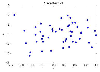
Matplotlib supports Matlab-style plotting commands, where you can quickly specify color (b for blue, r for red, k for black etc.) and a symbol for the plotting character ('-' for solid lines, '--' for dashed lines, '*' for stars, …)
In [60]:
s = np.arange(11)
plt.plot(s, s ** 2, 'r--')
Out[60]:
[<matplotlib.lines.Line2D at 0x687bd50>]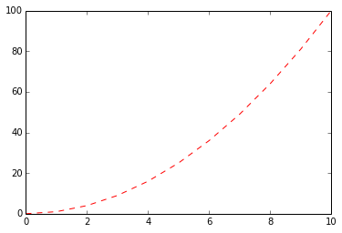
There is also a scatter command that also creates scatterplots
In [61]:
plt.scatter(x, y)Out[61]:
<matplotlib.collections.PathCollection at 0x667a390>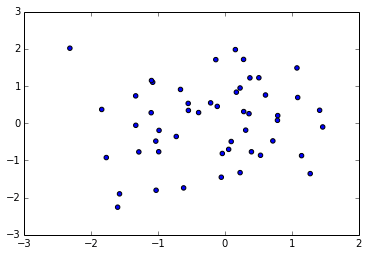
Boxplots are very useful to compare two distributionsIn [62]:
plt.boxplot([x, y])  # Pass a list of two arrays to plot them side-by-side
plt.title("Two box plots, side-by-side")
Out[62]:
<matplotlib.text.Text at 0x6155410>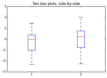
Matplotlib and Pandas
Pandas provides a convenience interface to matplotlib, you can create plots by using the pd.DataFrame.plot() method
In [63]:
# create a scatterplot of weight vs "miles per galone"
auto.plot(x='weight', y='mpg', style='bo')
plt.title("Scatterplot of weight and mpg")

# create a histogram of "miles per galone"
plt.figure()
auto.hist('mpg')
plt.title("Histogram of mpg (miles per galone)")
Out[63]:
<matplotlib.text.Text at 0x64e8190>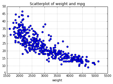
<matplotlib.figure.Figure at 0x6890c10>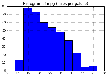
Finally, pandas has built in support for creating scatterplot matrices and much more.
In [64]:
from pandas.tools.plotting import scatter_matrix
_ = scatter_matrix(auto[['mpg', 'cylinders', 'displacement']], figsize=(14, 10))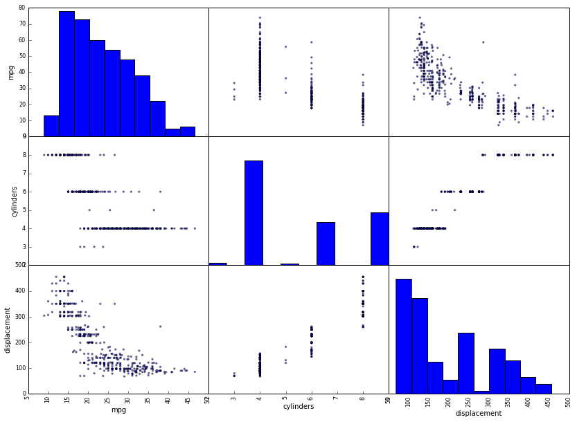
Matplotlib has a rich set of features to manipulate and style statistical graphics. Over the next few weeks we will cover many of them to help you make charts that you find visually appealing, but for now this should be enough to get you up and running in Python.
Further Reading
Python Scientific Lecture Notes
For a more in-depth discussion of the Python scientific computing ecosystem we strongly recommend the Python Scientific Lecture Notes. The lecture notes contain lots of code examples from applied science such as signal processing, image processing, and machine learning.
Wes Mckinney, the original author of pandas, wrote a great book on using Python for data analysis. It is not only the primary reference to pandas but also features a concise yet profound introduction to Python, numpy and matplotlib.

Download Notebook View on NBViewer
This post was written by Peter Prettenhofer and Mark Steadman. Please post any feedback, comments, or questions below or send us an email at <firstname>@datarobot.com.

This post was inspired from the StatLearning MOOC by Stanford.
-
Choosing the Right Vector Embedding Model for Your Generative AI Use Case
March 7, 2024· 8 min read -
Reflecting on the Richness of Black Art
February 29, 2024· 2 min read -
6 Reasons Why Generative AI Initiatives Fail and How to Overcome Them
February 8, 2024· 9 min read
Latest posts
Related Posts

You’ve just successfully subscribed


